Data Manipulation and Visualization in R

Nicolas Cardenas | March 11, 2026

---

Table of Contents

1. Introduction
2. Getting Started with RStudio
3. Installing and Loading Packages
4. Importing and Exploring Data
5. Data Manipulation with dplyr
6. Data Visualization with ggplot2
7. Saving and Exporting Your Work
8. Exercises

---

Introduction

Welcome! This tutorial will guide you through two of the most important skills in data analysis with R: manipulating data and creating visualizations. We will use a fun dataset — Pokémon stats — to practice these skills in an engaging way.

💡 Don't worry if something feels confusing. Even experienced R users search for help regularly. The goal here is to build your confidence through hands-on practice, not to memorize everything.

Why R?

R is a free, open-source programming language widely used in science, research, and medicine. In veterinary research, R helps you:

• Summarize large datasets (e.g., patient records, lab results)
• Identify patterns and trends in animal health data
• Create publication-quality charts and figures

What You Will Learn

By the end of this tutorial, you will be able to:

• Navigate the RStudio interface
• Load and explore a dataset
• Filter, summarize, and transform data using dplyr
• Create scatter plots, bar plots, histograms, and boxplots using ggplot2
• Save your data and plots to files

---

Getting Started with RStudio

Logging In (NCSU Students)

Go to Posit Workbench and log in with your UnityID and password.

The RStudio Interface

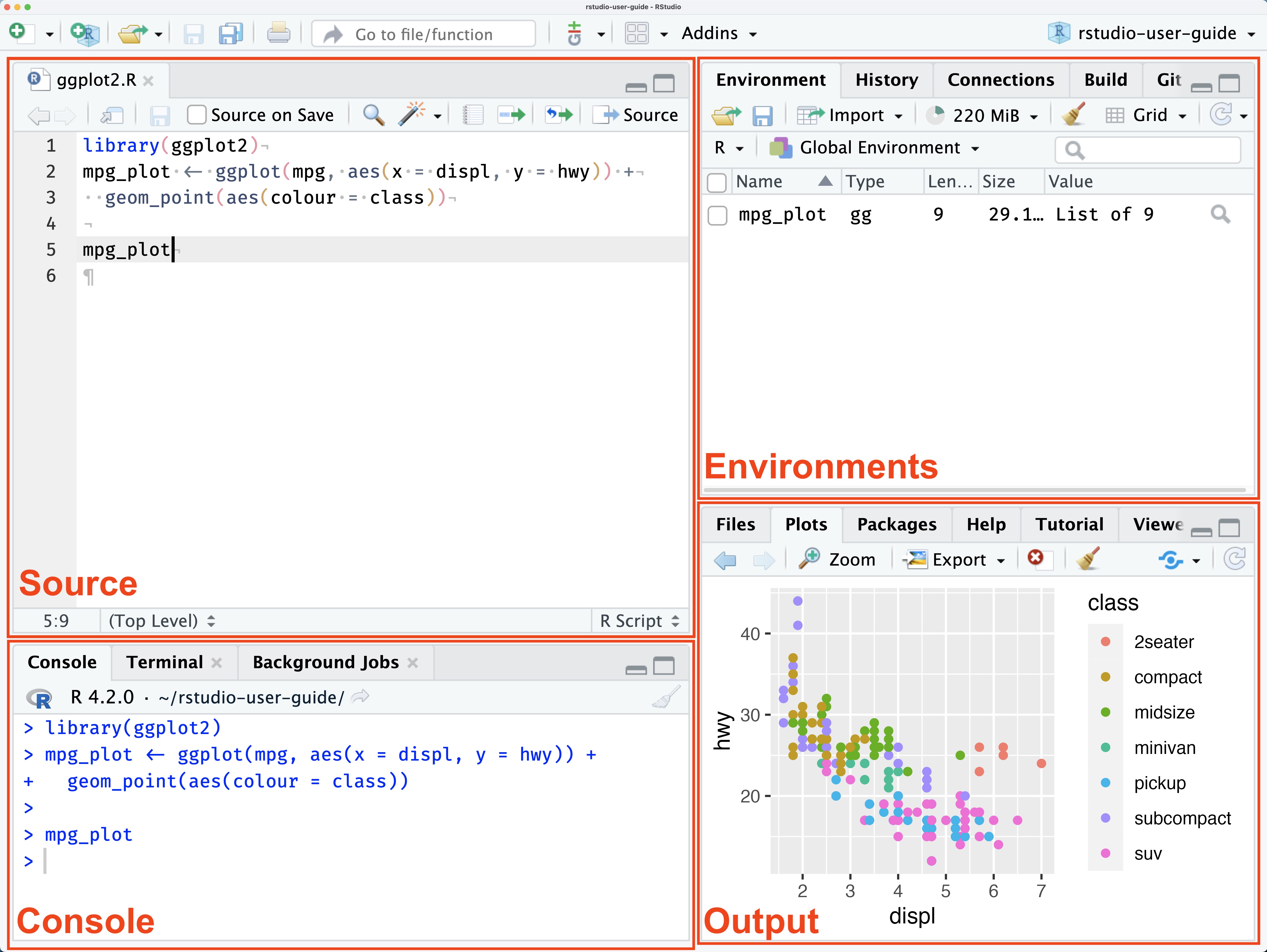
RStudio is divided into four main areas (called panes):

Pane	What it does
Source (top-left)	Write and save your R scripts here. Think of it as your notebook.
Environment (top-right)	Shows all the data and variables currently loaded in your session.
Console (bottom-left)	Where R actually runs your code. You can type commands here directly, or run them from the Source pane.
Output (bottom-right)	Displays your plots, help documentation, and file browser.

💡 Tip: Write your code in the Source pane so you can save and reuse it. Use the Console for quick, one-off commands.

---

Installing and Loading Packages

R's power comes from packages — collections of functions written by the community. Think of them like apps on your phone: you install them once, then load them each session.

# --- STEP 1: Install packages (run this ONCE, then comment it out) ---
install.packages("tidyverse")   # A bundle of data science packages
install.packages("pokemon")     # The Pokémon dataset

# --- STEP 2: Load packages (run this every time you start a new session) ---
library(tidyverse)   # Loads ggplot2, dplyr, and more
library(pokemon)     # Loads the Pokémon data

⚠️ Common mistake: You only need to install.packages() once. After that, just use library() to load the package at the start of each session. Installing every time wastes time and can cause errors.

What is the tidyverse?

The tidyverse is a collection of R packages designed to work together seamlessly. The two we'll focus on are:

• dplyr — for manipulating data (filtering, summarizing, creating new columns)
• ggplot2 — for creating visualizations

---

Importing and Exploring Data

Loading the Pokémon Dataset

The pokemon package contains a dataset with 949 Pokémon and 22 variables, including name, type, height, weight, HP, attack, defense, and more.

A full variable dictionary can be accessed here.

# Load the Pokémon data into your environment
pokemondata <- pokemon

# --- Ways to explore your data ---

glimpse(pokemondata)   # Quick summary: variable names, types, and first few values
View(pokemondata)      # Open the data in a spreadsheet-like viewer
nrow(pokemondata)      # How many rows (Pokémon)?
ncol(pokemondata)      # How many columns (variables)?
names(pokemondata)     # List all variable names
summary(pokemondata)   # Basic statistics for every column

💡 What is a data frame? In R, data is stored in a structure called a data frame — essentially a table with rows and columns, similar to an Excel spreadsheet. Each row is an observation (one Pokémon), and each column is a variable (e.g., hp, type_1, weight).

Understanding Variable Types

When you run glimpse(), you'll notice letters like <chr> and <dbl> next to variable names. These indicate the type of data stored in each column:

Type	Abbreviation	Example
Character (text)	<chr>	"fire", "Pikachu"
Double (number)	<dbl>	35.0, 120.5
Integer	<int>	1, 45
Logical	<lgl>	TRUE, FALSE

---

Data Manipulation with dplyr

dplyr provides a set of intuitive verbs (functions) for working with data. Each verb does one clear thing, and you can chain them together using the pipe operator (%>%).

💡 What is the pipe (%>%)? It means "take this, then do that." Instead of writing nested functions like arrange(filter(data, hp > 50)), you write data %>% filter(hp > 50) %>% arrange(hp) — much easier to read!

1. Selecting Columns with select()

Use select() to keep only the columns you need, or to drop columns you don't.

# Keep only specific columns (creates a new, smaller data frame)
poke_select <- pokemondata %>%
  select(pokemon, type_1, hp, attack, defense)

# Drop specific columns using the minus sign (-)
pokemondata <- pokemondata %>%
  select(-id, -url_image, -url_icon)   # Remove ID and image URL columns

💡 Why reduce columns? Large datasets with many variables can be hard to work with. Selecting only what you need makes your work cleaner and faster.

---

2. Filtering Rows with filter()

Use filter() to keep only rows that meet certain conditions.

# Keep only Pokémon with base experience greater than 200
high_exp_pokemon <- pokemondata %>%
  filter(base_experience > 200)

# Filter by type
fire_pokemon <- pokemondata %>%
  filter(type_1 == "fire")   # == means "is equal to"

# Combine multiple conditions with & (AND) or | (OR)
fire_or_water <- pokemondata %>%
  filter(type_1 == "fire" | type_1 == "water")   # | means OR

strong_fire <- pokemondata %>%
  filter(type_1 == "fire" & attack > 80)          # & means AND

Common comparison operators in R:

Operator	Meaning	Example
==	Equal to	type_1 == "fire"
!=	Not equal to	type_1 != "normal"
>	Greater than	hp > 100
<	Less than	weight < 10
>=	Greater than or equal	attack >= 90
<=	Less than or equal	defense <= 50

---

3. Creating New Columns with mutate()

Use mutate() to add new columns or modify existing ones.

# Add a new column converting weight from hectograms to kilograms
# (The Pokémon package stores weight in hectograms: 1 kg = 10 hg)
pokemondata <- pokemondata %>%
  mutate(weight_kg = weight / 10)

# Add a column categorizing Pokémon as "heavy" or "light"
pokemondata <- pokemondata %>%
  mutate(size_category = ifelse(weight_kg > 50, "heavy", "light"))

# Replace values in a column using replace()
modified_data <- pokemondata %>%
  mutate(type_1_new = replace(type_1, type_1 == "fire", "flame"))
  # Changes all "fire" entries to "flame" in a new column called type_1_new

💡 ifelse() explained: ifelse(condition, value_if_true, value_if_false). It checks the condition for every row and assigns the appropriate value.

---

4. Summarizing Data with group_by() and summarize()

Use group_by() combined with summarize() to calculate statistics for each group in your data.

# Group Pokémon by their primary type and compute summary statistics
summary_pokemon <- pokemondata %>%
  group_by(type_1) %>%                                              # Group by type
  summarize(
    count            = n(),                                         # Number of Pokémon per type
    avg_base_exp     = mean(base_experience, na.rm = TRUE),         # Average base experience
    max_height       = max(height, na.rm = TRUE),                   # Tallest Pokémon per type
    total_weight     = sum(weight_kg, na.rm = TRUE),                # Combined weight per type
    avg_attack       = mean(attack, na.rm = TRUE)                   # Average attack stat
  )

# View the result
summary_pokemon

💡 What does na.rm = TRUE mean? Some Pokémon might have missing values (NA) for certain stats. Setting na.rm = TRUE tells R to ignore those missing values when calculating. If you leave it out and there's even one NA, your result will also be NA.

---

5. Sorting Data with arrange()

# Sort by base experience, highest first (descending)
sorted_by_exp <- pokemondata %>%
  arrange(desc(base_experience))

# Sort by multiple columns: first by type, then by attack within each type
sorted_by_type_attack <- pokemondata %>%
  arrange(type_1, desc(attack))

---

Chaining It All Together

One of the most powerful features of dplyr is combining multiple verbs in a single pipeline:

# Full pipeline: filter, create a new column, group, summarize, then sort
result <- pokemondata %>%
  filter(!is.na(base_experience)) %>%             # Remove rows with missing experience
  mutate(weight_kg = weight / 10) %>%             # Add weight in kg
  group_by(type_1) %>%                            # Group by type
  summarize(
    count        = n(),
    avg_attack   = mean(attack, na.rm = TRUE),
    avg_weight   = mean(weight_kg, na.rm = TRUE)
  ) %>%
  arrange(desc(avg_attack))                       # Sort by highest average attack

---

Data Visualization with ggplot2

ggplot2 builds plots layer by layer. Every plot starts with ggplot(), then you add geoms (the visual shapes), aesthetics (what maps to x, y, color, etc.), and labels.

ggplot(data, aes(x = ..., y = ..., color = ...)) +
  geom_point() +      # the type of plot
  labs(...)           # titles and labels

💡 The + sign in ggplot2 adds layers to your plot — it is not the same as the %>% pipe. Think of %>% as "then do this to the data", and + as "then add this to the plot."

---

Plot 1: Scatter Plot

A scatter plot is great for exploring the relationship between two numeric variables.

# Scatter plot: Weight vs. Height, colored by primary type
ggplot(pokemondata, aes(x = weight, y = height, color = type_1)) +
  geom_point(size = 3, alpha = 0.7) +    # alpha controls transparency (0 = invisible, 1 = solid)
  labs(
    title  = "Pokémon Height vs. Weight",
    x      = "Weight (hg)",
    y      = "Height (dm)",
    color  = "Primary Type"
  ) +
  theme_minimal()   # A clean, simple background theme

Key arguments explained:

• aes(x = weight, y = height, color = type_1) — maps weight to the x-axis, height to the y-axis, and colors points by type
• size = 3 — controls how large each point is
• alpha = 0.7 — makes overlapping points slightly transparent so you can see them better
• theme_minimal() — removes the grey background for a cleaner look

---

Plot 2: Bar Plot

A bar plot is ideal for comparing a numeric value across categories.

# Bar plot: Average base experience by Pokémon type
# Note: This uses the summary_pokemon data frame we created earlier
ggplot(summary_pokemon,
       aes(x = reorder(type_1, avg_base_exp),   # reorder() sorts bars by value
           y = avg_base_exp,
           fill = type_1)) +
  geom_bar(stat = "identity", show.legend = FALSE) +   # stat="identity" uses the actual values
  coord_flip() +    # Flip horizontal for easier reading of type names
  labs(
    title = "Average Base Experience by Pokémon Type",
    x     = "Pokémon Type",
    y     = "Average Base Experience"
  ) +
  theme_minimal()

💡 stat = "identity" vs default: By default, geom_bar() counts rows. Using stat = "identity" tells it to use the actual y-values in your data instead — which is what you want when plotting summary statistics.

---

Plot 3: Histogram

A histogram shows the distribution of a single numeric variable — how values are spread out.

# Histogram: Distribution of base experience across all Pokémon
ggplot(pokemondata, aes(x = base_experience)) +
  geom_histogram(
    binwidth = 20,        # Each bar covers a range of 20 experience points
    fill     = "steelblue",
    color    = "black",   # Outline color of each bar
    alpha    = 0.7
  ) +
  labs(
    title = "Distribution of Pokémon Base Experience",
    x     = "Base Experience",
    y     = "Number of Pokémon"
  ) +
  theme_minimal()

💡 Choosing binwidth: Too small a binwidth makes the plot noisy and hard to read; too large hides important patterns. Try a few values (e.g., 10, 20, 50) to find what looks best for your data.

---

Plot 4: Boxplot

A boxplot summarizes the distribution of a variable across groups, showing the median, spread, and outliers.

# Boxplot: Base experience by Pokémon type
ggplot(pokemondata,
       aes(x = reorder(type_1, base_experience, median),  # Sort by median experience
           y = base_experience,
           fill = type_1)) +
  geom_boxplot(
    outlier.shape = 21,      # Shape of outlier points
    outlier.fill  = "red",   # Fill outliers red so they stand out
    outlier.size  = 2,
    alpha         = 0.7
  ) +
  coord_flip() +
  labs(
    title = "Base Experience Distribution by Pokémon Type",
    x     = "Pokémon Type",
    y     = "Base Experience"
  ) +
  theme_minimal() +
  theme(legend.position = "none")   # Hide legend (color already shown on axis)

Reading a boxplot:

         |-----|=====|=====|-----|    o  (outlier)
         Min  Q1   Median  Q3   Max

• The box shows the middle 50% of values (Q1 to Q3)
• The line inside the box is the median
• The whiskers extend to the min/max within 1.5× the interquartile range
• Dots beyond the whiskers are outliers

---

Saving and Exporting Your Work

Save Your Data

# Save as a CSV file (universally compatible)
write_csv(pokemondata, "pokemon_data.csv")

# Save as an Excel file
library(writexl)
write_xlsx(pokemondata, "pokemon_data.xlsx")

Save Your Plots

# Save the most recently displayed plot
ggsave("my_plot.png", dpi = 300, width = 8, height = 6)
# dpi = 300 gives print-quality resolution
# width and height are in inches

# Save a specific plot object
my_plot <- ggplot(pokemondata, aes(x = weight, y = height)) + geom_point()
ggsave("weight_vs_height.png", plot = my_plot, dpi = 300, width = 8, height = 6)

💡 Where does the file save? By default, R saves to your working directory. Check where that is with getwd(), and change it with setwd("path/to/folder").

---

Exercises

Work through the following exercises using the skills from this tutorial. For each exercise, write your code in an R script (.R file) and comment your work so someone else could understand what you did.

---

Exercise 1 — Visualizing Attack Stats by Type

Create a plot that compares the Attack stat across Pokémon primary types (type_1).

Hints:

• A boxplot or bar plot would work well here
• Use group_by() + summarize() if you want average attack per type
• Label your axes clearly and add a title

Challenge: Add color by type and sort the plot so the type with the highest attack appears at the top.

---

Exercise 2 — How Many Pokémon Can Gengar Defeat?

Gengar's Special Attack stat is 130. Assume Gengar can defeat any Pokémon whose Special Defense stat is strictly less than 130.

Part A: How many Pokémon can Gengar defeat? Display the count in a table.

Part B: How many of those Pokémon are from each primary type? Display the results as a table sorted from most to fewest.

---

Exercise 3 — The Most Powerful Pokémon

Identify the most powerful Pokémon in the dataset. This is an open-ended question — there is no single right answer!

Your analysis must include:

1. A clear definition of "most powerful" (e.g., highest total stats? best attack/defense ratio? most wins?)
2. At least two visualizations supporting your conclusion
3. At least one summary table with relevant statistics
4. A written justification (3–5 sentences) explaining your reasoning

Some ideas to explore:

• Create a total_stats column by summing hp + attack + defense + special_attack + special_defense + speed
• Compare distributions across types
• Look at outliers in your boxplots — who are those dots?

---

Bonus — Explore on Your Own

Visit https://www.data-to-viz.com/ for inspiration on chart types and when to use them:

Choose one chart type not covered in this tutorial and recreate it using the Pokémon dataset. Include a brief explanation of why that chart type is useful for the variable(s) you chose.

---

For a variable dictionary, see the pokemon package documentation.