MiniTorch

A compact NumPy neural-network framework with fast reverse-mode autograd, a compiled dense-training loop, and an interactive scientific model explorer. MiniTorch keeps the implementation small enough to study while providing a practical API for experiments.

Highlights

• Linear-time reverse execution tape for first-order backpropagation.
• Raw NumPy gradient kernels avoid constructing temporary autograd graphs.
• Familiar Variable, Module, Sequential, Linear, activation, and optimizer APIs.
• Optional Cython-generated C loop for dense classifier training; NumPy still provides optimized matrix multiplication.
• Self-contained React full-neuron model explorer.
• Higher-order differentiation remains available with backward(create_graph=True).

Install

Python 3.10 or newer is required. Release wheels target Linux x86-64, Windows x64, and 64-bit Intel/Apple silicon macOS.

pip install minitorchbr

For development or to compile the native trainer from source:

git clone https://github.com/BriceLucifer/MiniTorch.git
cd MiniTorch
uv venv
uv sync

Source installation requires a C/C++ build toolchain because the native trainer is compiled during installation.

Autograd

import numpy as np
from MiniTorch import Variable

x = Variable(np.array([[2.0]], dtype=np.float32), name="x")
w = Variable(np.array([[3.0]], dtype=np.float32), name="w")
b = Variable(np.array([[1.0]], dtype=np.float32), name="b")

loss = (x * w + b - 10.0) ** 2
loss.backward()

print(loss.data)    # [[9.]]
print(x.grad.data)  # [[-18.]]
print(w.grad.data)  # [[-12.]]
print(b.grad.data)  # [[-6.]]

The normal backward path traverses each graph node and edge once. Pass create_graph=True when the backward computation itself must remain differentiable.

Build a model

from MiniTorch.nn import Linear, ReLU, Sequential

model = Sequential(
    Linear(64, 128),
    ReLU(),
    Linear(128, 64),
    ReLU(),
    Linear(64, 10),
)

print(model)
print(model.summary())

Eager training

Use eager mode for arbitrary modules, custom operations, dynamic model code, or higher-order gradients:

from MiniTorch import Variable
from MiniTorch.ops import softmax_cross_entropy
from MiniTorch.optim import Adam

optimizer = Adam(model.parameters(), lr=1e-3)

for features, labels in loader:
    logits = model(Variable(features))
    loss = softmax_cross_entropy(logits, Variable(labels))

    optimizer.zero_grad()
    loss.backward()
    optimizer.step()

Compiled training loop

For a static Sequential(Linear, ReLU, ..., Linear) classifier, train moves the epoch, mini-batch, forward, backward, softmax cross-entropy, and Adam loops out of Python:

from MiniTorch.native import train

history = train(
    model,
    x_train,
    y_train,
    epochs=15,
    batch_size=128,
    lr=1e-3,
)

print(history.losses[-1])

Inputs and parameters use contiguous float32; labels use integer class indices. Parameters are updated in place, and gradients from the final batch remain attached for inspection. Unsupported model structures should use eager training.

Interactive model visualization

The public API is intentionally small:

from MiniTorch import visualize

visualize(model)

This writes model_architecture.html and opens a self-contained interactive viewer. No server is required.

result = visualize(
    model,
    filename="artifacts/model.html",
    input_shape=(None, 64),
    open_browser=False,
)
print(result.path)

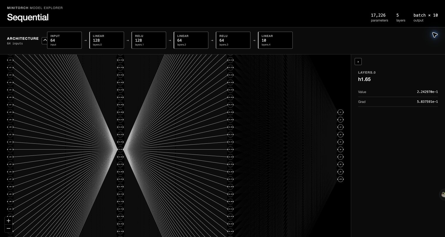
The viewer provides:

• every neuron in every dense layer—no representative sampling;
• a canvas-rendered full connection mesh that remains responsive at high edge counts;
• a separate compact architecture overview above the neuron map;
• map-style zoom and pan plus slim horizontal and vertical scrollbars;
• a fixed, distraction-free black scientific theme;
• independent collapse controls for the architecture and inspector;
• a deliberately small neuron inspector containing only Value and Grad.

Value is captured by the latest eager forward pass. Use loss.backward(retain_grad=True) before visualize(model) to retain hidden activation gradients for Grad.

import numpy as np

from MiniTorch import Variable, sum as tensor_sum, visualize

probe = Variable(np.random.default_rng(7).normal(size=(1, 64)).astype(np.float32))
probe_output = model(probe)
probe_loss = tensor_sum(probe_output)
probe_loss.backward(retain_grad=True)
visualize(model)

The exporter is shape-driven rather than tied to the example above. A single-layer 10 → 1 network produces exactly 10 input neurons, one output neuron, and 10 connections:

from MiniTorch import visualize
from MiniTorch.nn import Linear, Sequential

small_model = Sequential(Linear(10, 1))
visualize(small_model, filename="small-model.html")

To rebuild the bundled frontend after editing it:

cd lib/graph-viewer
npm ci
npm run typecheck
npm run build

The generated JavaScript and CSS are packaged under MiniTorch/visualization/static/.

Autograd graph debugging

Use the separate computation-graph viewer to inspect one expression:

from MiniTorch import visualize_graph

loss.backward(retain_grad=True)
visualize_graph(loss, filename="autograd_graph.html")

Examples

All examples run from the repository root:

uv run python examples/basic_autograd.py
uv run python examples/native_training.py
uv run python examples/model_visualization.py
uv run python examples/autograd_graph.py
uv run python examples/mnist.py

examples/mnist.py downloads MNIST on first use, trains it through the compiled loop, evaluates the result, and opens the trained network in the model explorer.

Performance

The benchmark scripts compare graph traversal and complete training paths:

uv run python benchmarks/benchmark_autograd.py
uv run python benchmarks/benchmark_native_training.py
uv run python benchmarks/benchmark_autograd.py --quick --json

Latest local smoke results (Python 3.14.3, NumPy 2.4.3, Apple silicon):

Benchmark	Median
Backward through a 2,000-node chain	5.20 ms
Backward through 1,000 fan-out branches	5.54 ms
Dense MLP training, batch 256	1.28 ms / 199,740 samples/s
Compiled loop versus eager training	1.74× faster

Results depend on CPU, NumPy build, BLAS library, and workload. Run the included benchmarks on the target machine; quick-mode samples are smoke measurements, not fixed performance guarantees.

Repository layout

MiniTorch/
├── core/              Variable, Function, and gradient configuration
├── ops/               differentiable NumPy operations
├── nn/                modules, dense layers, activations, containers
├── optim/             SGD and Adam
├── native/            compiled dense-classifier training loop
├── visualization/     model exporter and packaged web viewer
├── data/              MNIST loader and mini-batch DataLoader
└── utils/             graph tools, plots, and numerical checks
benchmarks/             reproducible performance measurements
docs/                   MkDocs Material documentation
examples/               runnable focused examples
lib/graph-viewer/       React and TypeScript viewer source
tests/                  correctness and integration tests

Generated plots and demo outputs are deliberately not committed. Examples write their artifacts into the current working directory.

Development

uv sync
uv run pytest tests/ -q
uv run mypy MiniTorch

cd lib/graph-viewer && npm ci && npm run typecheck && npm run build
cd ../..
uv run --group docs mkdocs build --strict
uv build

Documentation

The full guide covers installation, training, and model visualization.

License

MiniTorch is released under the MIT License.